Climate model
Introduction
The purpose of this page is to introduce some tools that allow climate modeling in an educational context or learn basic climate modeling principles and/or techniques. At some later point we plan to add educational questions...
Modeling principles
Climate models use standard modeling techniques, but often adapted to the specific requirements of modeling climate. There exist several free tools for education that allow learning various modeling principles, e.g. NetLogo includes agent-based simulation and systems dynamics (difference equations).
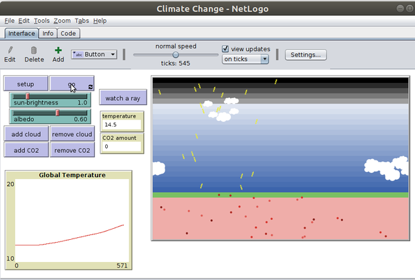
The software also includes a little climate simulation model [1] that could be used in a school context to explain how simulations work.
The model is implemented as agent-based simulation: “Yellow arrowheads stream downward representing sunlight energy. Some of the sunlight reflects off clouds and more can reflect off the earth’s surface. If sunlight is absorbed by the earth, it turns into a red dot, representing heat energy. Each dot represents the energy of one yellow sunlight arrowhead. The red dots randomly move around the earth, and its temperature is related to the total number of red dots. Sometimes the red dots transform themselves into infrared (IR) light that heads toward space, carrying off energy.” ("How it works") [1]
This model allows learning the general global logic. Learners (end users) can play with the following parameters.
- SUN-BRIGHTNESS (1 corresponds to our sun)
- ALBEDO, how much of the sun energy hitting the earth is absorbed. The Earth's albedo is about 0.6
- Clouds can be added or removed
- Greenhouse gases (i.e. CO2 molecules) can be added or removed
It is important to understand that this is not a realistic simulation the earth's climate, but it can explain important modeling principles and also the role of important parameters in a climate model.
Monash university simple climate model
The model
The Monash simple climate model home page [2] explains the model, includes some tutorials and allows to play with different scenarios and also to deconstruct models by switching offf some processes. According to the web site (retrieved April 2019), “the Monash simple climate model (MSCM) is based on the Globally Resolved Energy Balance (GREB) model, which is a physical climate model published by Dommenget and Floeter [2011] [3] in the international peer review science journal Climate Dynamics. The model simulates most of the main physical processes in the climate system in a very simplistic way and therefore allows very fast and simple climate model simulations on a normal PC computer. It simulates the global climate on gird of 96 times 48 points on three different vertical levels (surface, atmosphere and subsurface ocean). Despite its simplicity the model simulates the climate response to external forcings, such as doubling of the CO2 concentrations very realistically (similar to state of the art climate models)”
The GREB model can be summarized with the following tendency equation:
- The meaning of each term is explained int the Dommenget & Flöter (2011) article [3]
The Monash simple climate model website includes both resources and interfaces allowing to play with the model. An alternative website suggested for European users is mscm.dkrz.de/. It also is possible to run the software on your own server.
Model interfaces
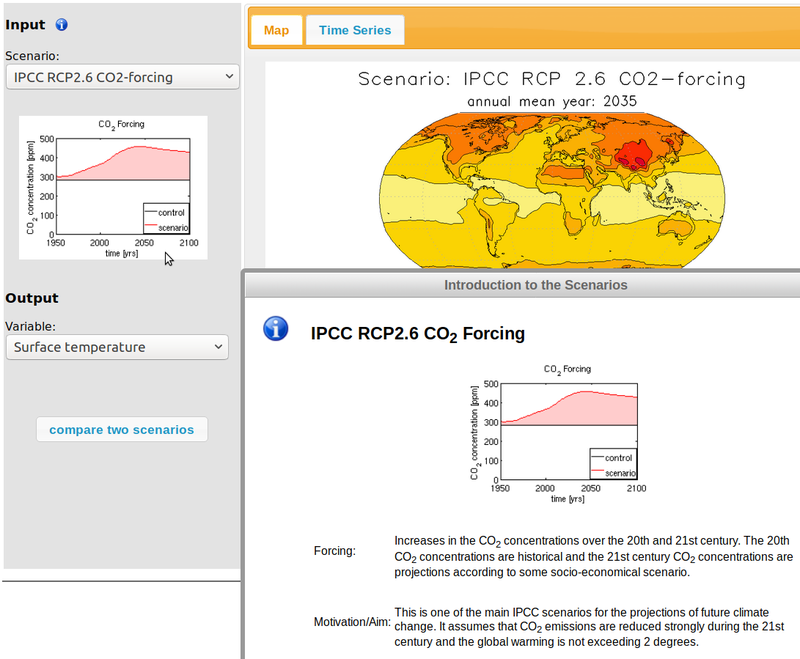
One included tool allows playing with various scenarios with respect to CO2 emission. The following screen capture shows the climate change scenarios interface. It allows visualizing the effect of some published (?) scenarios and one could compare two of these.

The deconstruction tools allow seeing what happens if one omits one or more parameters from the model. “In this interface you can deconstruct the Monash simple climate model by switching ‘OFF’ processes of the model. This will allow you to learn how the different processes in the climate interact to create the complex mean state climate as it is observed. The Interface can be used in two different complexity levels:” a 11 parameter standard version for students with a a climate physics backgrand and a six parameter basic version for school students.
For example, in the Deconstruct the Mean Climate interface, shown in the next screenshot, we removed ice albedo (reflection) and as result got more warming.
The next screenshot shows two experiments with the standard version of the Deconstruct the Response to 2xCO2 interface.
“In this interface [one] can deconstruct the Monash simple climate model response to doubling of the CO2 concentrations by switching ‘OFF’ processes of the model. This will allow you to learn how the different processes in the climate interact to create the complex climate response to anthropogenic CO2 emissions”. There are two complexity variants, a standard version with 10 parameters and a basic version with 5. The standard version allows for about 200 different experiments (not all on/off combinations are modeled). Version B without the hydrological cycle shows less warming of the surface temperature.
Tutorials
The web site include some walk-through tutorials that explain how to use the model interface and also provide background information. Popup blockers in your navigator must be disabled for this web site.
Professional environments
Professional environments also can be used in education, in particular in more advanced classes. But they do require an expert teacher. A number of open source and free environments exist. Below, a selection.
Apache Open Climate Workbench
The Apache open climate workbench (OCW) allows playing with climate models and data from various sources, e.g. creating visualizations. Installation of this software may require some system administration skills. There is a simplified installation procedure for Ubuntu (dated 2015). We did not test to install OCW so far.
According to the project home page (April 2019), “Apache Open Climate Workbench is an effort to develop software that performs climate model evaluation using model outputs from a variety of different sources the Earth System Grid Federation, the Coordinated Regional Climate Downscaling Experiment, the U.S. National Climate Assessment and the North American Regional Climate Change Assessment Program and temporal/spatial scales with remote sensing data from NASA, NOAA and other agencies. The toolkit includes capabilities for rebinning, metrics computation and visualization.”
Another, older, definition of the project is on the Open Climate Workbench documentation platform: “The Apache Open Climate Workbench(OCW) is a comprehensive suite of algorithms, libraries, and interfaces designed to standardize and streamline the process of interacting with large quantities of observational data [...] and conducting regional climate model evaluations.”. Furthermore, “OCW consists of a Python library for common model evaluation tasks (e.g. area averaging, regridding, bias calculation) as well as a set of user-friendly interfaces for quickly configuring a large-scale regional model evaluation task. Users can interact with the OCW either by including the Python library directly in their code, or by way of the flexible RESTful Application Programmer Interface (API).” That means that this library also could run as web service.
M.I.T General Circulation Model
The MITgcm (MIT General Circulation Model) is a numerical model designed for study of the atmosphere, ocean, and climate. Its non-hydrostatic formulation enables it to simulate fluid phenomena over a wide range of scales; its adjoint capability enables it to be applied to parameter and state estimation problems. By employing fluid isomorphisms, one hydrodynamical kernel can be used to simulate flow in both the atmosphere and ocean.
The software is free and available on GitHub. Using it requires advanced modeling skills.
Isca framework for idealised global circulation modelling
“Isca is framework for the idealized modelling of the global circulation of planetary atmospheres at varying levels of complexity and realism. The framework is an outgrowth of models from GFDL designed for Earth's atmosphere, but it may readily be extended into other planetary regimes.” (about)
The purpose of this framework extends prediction of earth's climate. “Understanding climate is not synonymous with predicting or simulating climate. In order to provide the best possible predictions of Earth's weather and climate we need comprehensive models that provide simulations with the greatest possible degree of verisimilitude.”
The model, also allowing climate modelling of some other planets, has been described in Vallis et al. (2017) [4] and is available on GitHub.
Links
Official MSCM servers
Other
On climate change
There are many Wikipedia pages on climate change and climate modeling. For example:
- Portal:Global warming
- Climate change
- Global warning (main article)
The conversation has several interesting articles on climate science, some of which point to open source models and software.
- Articles on climate science, e.g. Making climate models open source makes them even more useful by Martin Jucker.
Bibliography
- ↑ 1.0 1.1 Tinker, R. and Wilensky, U. (2007). NetLogo Climate Change model. http://ccl.northwestern.edu/netlogo/models/ClimateChange. Center for Connected Learning and Computer-Based Modeling, Northwestern University, Evanston, IL.
- ↑ The Monash Simple Climate Model Experiments: An interactive database of the mean climate, climate change and scenarios simulations by Dietmar Dommenget, Kerry Nice, Tobias Bayr, Dieter Kasang, Christian Stassen and Mike Rezny, submitted in 03/2018 to Geoscientific Model Development
- ↑ 3.0 3.1 Dietmar Dommenget and Janine Flöter (2011), Conceptual Understanding of Climate Change with a Globally Resolved Energy Balance Model, Journal of Climate Dynamics 37: 2143. doi:10.1007/s00382-011-1026-0
- ↑ Vallis, G. K., Colyer, G., Geen, R., Gerber, E., Jucker, M., Maher, P., … Thomson, S. I. (2018). Isca, v1.0: a framework for the global modelling of the atmospheres of Earth and other planets at varying levels of complexity. Geoscientific Model Development, 11(3), 843–859. https://doi.org/10.5194/gmd-11-843-2018


